EDM: Electron Direct Methods
EDM is a set of programs intended to combine various aspects of image processing and manipulation of high resolution images and diffraction patterns as well as direct methods. Two additional programs are distributed with the code, NCEMSS which is a multislice package and MBFIT which is a beta version of code for CBED simulation. The intent is to make available to the general user a relatively simple user-interface mouse driven version of what has been to date research oriented code. The code is Public Domain under the standard GNU license, which means that it is free to use or modify for non-commercial purposes.
The full functionality of the software is relatively large, and includes:
This program is distributed in the hope that it will be useful, but WITHOUT ANY WARRANTY; without even the implied warranty of MERCHANTABILITY or FITNESS FOR A PARTICULAR PURPOSE. See the GNU General Public License for more details.
Because this program is licensed free of charge, there is no warranty for the program, to the extent permitted by applicable law. Except when otherwise stated in writing the copyright holders and/or other parties provide the program "as is" without warranty of any kind, either expressed or implied, including, but not limited to, the implied warranties of merchantability and fitness for a particular purpose. The entire risk as to the quality and performance of the program is with you. Should the program prove defective, you assume the cost of all necessary servicing, repair or correction.
1. Getting Started
1.1 The Control Panel
1.2 Command-line Options
2. Operating on an Image
2.1 Tools and Filters
2.2 Image Symmetry Analysis
2.3 Potential Map Tool
3. Quantifying a Diffraction Pattern
3.1 Defining the Lattice
3.2 Peak Quantification
5. Running Direct Methods -- (fs98)
5.1 Convergence Analysis
5.2 Genetic Analysis
5.3 Analyzing the Direct Methods Results
7. Maximum Entropy and Wiener Deconvolution
8. An Exercise
8.1 Analysis of Images
8.2 Direct Methods
9. Installation
9.1 Notes About the Win32 Version
10. Menus and Submenus
10.1 File Menu
10.2 Edit Menu
10.3 Process Menu
10.4 Direct Methods
10.5 Windows
12. FAQ: Frequently Asked Questions
13. Detailed Command Information
 Before you launch into using EDM, you want to setup for yourself a directory where you will work. In this directory (it does not have to be, but for convenience) you should have whatever diffraction patterns and images you want to analyze. At present the program can handle tiff images, as well as raw data in a variety of forms. (As a caveat, files written using line-based FORTRAN code can be difficult; there is a question of how many additional characters there are at the end of a line, typically two.)
You next want to ensure that you have your PATH variable set correctly, in general via a command such as
export PATH=$PATH:/usr/local/edm/bin, or
setenv PATH /user/local/edm/bin:$PATH
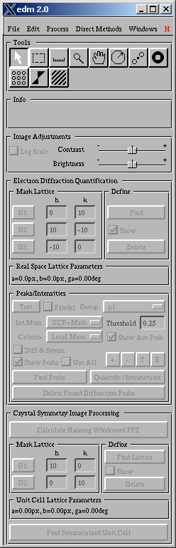
where "/usr/local/edm/bin" is the default location for the executable files but might be different with your installation. After this you are ready to go: just type "edm" at a terminal connected to an X display. This should bring up the main window, shown on the right. If it does not, you may have some environmental variables set wrong, or you do not have permissions.
For the Windows version of the software, you first need to start the X-server from the Windows Start Menu (Xwin). An ![]() icon should appear in your Windows taskbar signifying that an X-server is running. Then select EDM from the Start Menu to start EDM. (If the X-server does not start, you will need to get it to work before you will be able to use EDM. Alternatively, you can use a third-party X-server for this purpose.)
icon should appear in your Windows taskbar signifying that an X-server is running. Then select EDM from the Start Menu to start EDM. (If the X-server does not start, you will need to get it to work before you will be able to use EDM. Alternatively, you can use a third-party X-server for this purpose.)
CAVEAT: If your computer does not give you error messages and other information in English, this might cause problems with reading and writing files because the character set is larger than what the code expects (i.e. each character is two bytes). You may need to set the environmental variable LC_ALL=C or LC_ALL=en_US. This might happen if your computer speaks Russian, Japanese or Chinese.
The main control panel is divided into four major parts. The menu bar is used for general file control, window management, and access to features, and for launching the Direct Methods subprogram. Within the graphical section are three subsections. The top portion containing Tools, Info, and Image Acquisition has some basic image processing tools and can be used to edit the image and control the behavior of some of the other operations the software suite can perform, such as limiting acquisition of intensities to only those within a circular region. The second section, containing Electron Diffraction Quantification and Peaks/intensities, is used for acquisition of intensities from diffraction patterns. The last subsection, Crystal Symmetry Image Processing, is useful for processing real space images to gather phases or perform general analyses.
Some general points about fields, which window(s) are currently being operated on, and file formats. To edit any particular field, in general you click to edit them with the exception of tables in which you must double-click to edit. Copy and paste are available on various data columns. However, the copy/paste buffers are local to the program and are not exportable.
Operations are performed on the currently active window. You can change which window is active by clicking on its top bar. On some systems, the window may not activate if you click on it only once (for example, you might switch from an image to a table of reflections using one mouse click, and when saving the table you have actually saved the image that was previously selected rather than the dataset). In this case, activate the Click-To-Focus option under the Edit menu. Click-To-Focus is also useful for situations where EDM is running in an X-terminal because it causes the graphical buffers to refresh automatically.
Most files, for instance images, have standard naming conventions (e.g. XYZ.tif) which you should probably follow. For some of the files used in the Direct Methods analysis, a different approach common in crystallography is used. For different files the naming convention is prefix.suffix where prefix corresponds to a particular data set, and suffix varies with what the file is used for. For instance, MYRUN.hkl would correspond to a reflection dataset for MYRUN, whereas MYRUN.ins would have control information. More details can be found in the section on file formats.
When opening an image file, the software will prompt you for raw data import specifications if the filename is not recognized (i.e., not .tif). For dataset files, the extension must be .hkl or the program will not open it.
EDM has several command-line options for bug-fixing or diagnostics. The table below shows the options and their use:
| -d | Debug mode. Verbose output of program execution status and windowing behavior. |
| -h | Help info. Shows valid command-line flags for EDM (incomplete at this time). Does not launch EDM. |
| -t | Image test mode. Displays a 24-bit RGB/grayscale montage for testing your system's color capabilities. |
| -v | Verify mode. Displays the startup color options (i.e., bit depth, colormap, etc). |
| -cf | Sets click-to-focus on (default without -cf is off). You can also change this option when running EDM using the click-to-focus option in the Edit menu. |
NCEMSS command-line options are shown below:
| -a "number" | Where "number" is the maximum number of atoms. |
| -d "number | Where number is a power or 2 between 32->2048, the maximum array size. |
| -h | Will give information about help flags. |
| -s "size" | Where "size" is small, medium or large. |
| -v | Verbose |
EDM includes in its control panel a number of powerful tools for image processing. Details on how to use each of these are given below. Multiple operations on the image can be conducted serially to achieve desired results.
![]() Selection Tool - Allows you to select elements in the image such as masks and modify or delete them.
Selection Tool - Allows you to select elements in the image such as masks and modify or delete them.
![]() Rectangular Marquee - Used to select a rectangular area of the image for processing. Hold down the shift button while sizing the box to create a square marquee. One can use this tool to copy a portion of the original image to a new image via the copy, then paste options under the Edit menu. Operations such as FFT and Hanning Windowed FFT should be performed using square marquee.
Rectangular Marquee - Used to select a rectangular area of the image for processing. Hold down the shift button while sizing the box to create a square marquee. One can use this tool to copy a portion of the original image to a new image via the copy, then paste options under the Edit menu. Operations such as FFT and Hanning Windowed FFT should be performed using square marquee.
![]()
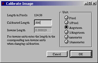 Line/Measure Tool - This tool is used for calibrating the image. Draw a line about a feature of known size, then select Calibrate in the Edit menu. This will bring up the "Calibrate Image" window (right) where you can specify the corresponding distance in real or reciprocal units. It is best to calibrate the image first, future processing will use these calibration measurements once the image has been calibrated. For a full structure analysis using both experimental phases and intensities, you will want to calibrate both the real space image and diffraction pattern before you begin the analysis.
![]() Magnify Tool - This tool allows you to zoom in on the image. Shift-clicking will zoom you out. Double-click will restore the image to its original 1x magnification and re-center it in the window (useful if you had used the move tool and the image has become off-center).
Magnify Tool - This tool allows you to zoom in on the image. Shift-clicking will zoom you out. Double-click will restore the image to its original 1x magnification and re-center it in the window (useful if you had used the move tool and the image has become off-center).
![]() Move Tool - You can move an image around in the window by clicking and holding the left mouse button. Useful for investigating regions of highly magnified images.
Move Tool - You can move an image around in the window by clicking and holding the left mouse button. Useful for investigating regions of highly magnified images.
![]() Processing Mask - This circular mask limits the boundaries under which EDM investigates image data. Use this to prevent out-of-picture errors during peak acquisition or prevent EDM from considering reflections outside of a certain radius. Place it by left-clicking at the desired radial limit of the mask. At this time the tool does not allow re-sizing of the mask; placing a new one will erase the old one.
Processing Mask - This circular mask limits the boundaries under which EDM investigates image data. Use this to prevent out-of-picture errors during peak acquisition or prevent EDM from considering reflections outside of a certain radius. Place it by left-clicking at the desired radial limit of the mask. At this time the tool does not allow re-sizing of the mask; placing a new one will erase the old one.
![]() Spot Mask - This can be used to select centrosymmetric pairs of reflections or groups of reflections by using a pair of circular masks.
Spot Mask - This can be used to select centrosymmetric pairs of reflections or groups of reflections by using a pair of circular masks.
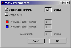
![]() Circular Mask - This centered mask is useful for band-pass filtering. The Edit Mask option in the "Process" menu contains options for smoothing out the mask and inverting its frequency passing functionality (the Opaque option). By default, the passband is in between the rings. You can do high-pass or low-pass filtering by dragging one of the rings outside of the image, sizing the remaining ring, and selecting the Opaque option for low-pass filtering (or de-selecting opaque for high-pass). Apply the mask using the Apply Mask option under the "Process" menu. A new pattern with the passed which can then be inverse Fourier transformed (also under the "Process" menu).
Circular Mask - This centered mask is useful for band-pass filtering. The Edit Mask option in the "Process" menu contains options for smoothing out the mask and inverting its frequency passing functionality (the Opaque option). By default, the passband is in between the rings. You can do high-pass or low-pass filtering by dragging one of the rings outside of the image, sizing the remaining ring, and selecting the Opaque option for low-pass filtering (or de-selecting opaque for high-pass). Apply the mask using the Apply Mask option under the "Process" menu. A new pattern with the passed which can then be inverse Fourier transformed (also under the "Process" menu).
![]()
 Lattice Mask - The lattice mask can be used to filter out the information in between reciprocal lattice spots, such as noise content in an image. This is also helpful in cases where two grains overlap and you want to separate two sets of lattice fringes. After placing the initial lattice mask pattern, select the lattice point size to be passed using the controls on the center circle. Rotate the lattice arrows to correspond to multiples of the h and k unit vectors. Next ctrl-click the head of each lattice arrow to increase the number of lattice rows to correspond to the lattice of interest. Shift-click reduces the number of lattice points within the lattice arrow (this is sometimes flaky). Refine the lattice using the arrowheads so that the circles correspond to reciprocal lattice points. The mask opacity and gradation can be modified similarly to the circular mask. Apply the mask, and perform the inverse Fourier transform to achieve the filtered image.
![]() Wedge Mask - This mask can segment the pattern into opposite wedges. Use the arrowheads to move the boundaries to their desired locations. The opacity option (discussed in circular mask section) can be used to swap the filtered and unfiltered regions.
Wedge Mask - This mask can segment the pattern into opposite wedges. Use the arrowheads to move the boundaries to their desired locations. The opacity option (discussed in circular mask section) can be used to swap the filtered and unfiltered regions.
![]() Grating Mask - This applies a parallel grating to the image that can be used to filter reciprocal lattice points arranged in parallel rows. Use the long arrowhead to rotate the grating, and the short arrowheads to specify grating spacing. Use Edit Mask in the Edit menu to widen the lines into parallel bands that will be passed in the inverse Fourier transform of the reciprocal space image.
Grating Mask - This applies a parallel grating to the image that can be used to filter reciprocal lattice points arranged in parallel rows. Use the long arrowhead to rotate the grating, and the short arrowheads to specify grating spacing. Use Edit Mask in the Edit menu to widen the lines into parallel bands that will be passed in the inverse Fourier transform of the reciprocal space image.
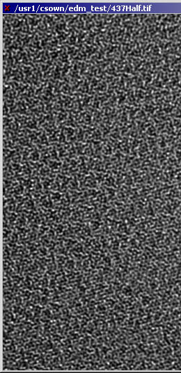
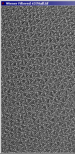
Some other useful tools and filters are also built into the code (under the Process menu). For instance, the Convert option allows you to change a complex image into a real image, phase image, intensity image, and others. Another powerful tool is a Wiener filter for reducing the effects of background noise, as illustrated below in the before image (left) and the filtered image (right).
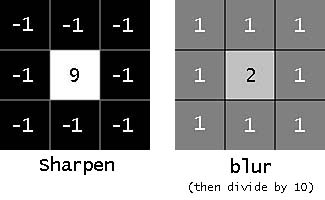
The Process menu also contains basic sharpen and blur functions. The filter kernels used for these operations are shown below:
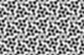
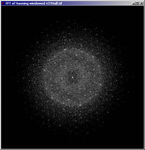
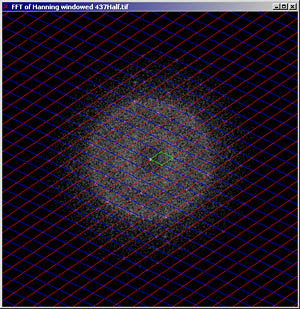
There are two different forms of Fourier transforms available. The first is a simple one without any mask applied (under the Process menu). This suffers from the problem of producing streaks (due to edge effects). A better implementation is to use a Hanning window, which avoids streaking by applying a specially gradated radial mask that yields diffraction-peak-like shape functions in reciprocal space that are easy for the algorithm to measure to great accuracy. In addition, by using a Hanning window, amplitudes and phases are extracted with greater precision. At the moment only the simple Fourier transform can be used to, for instance, apply a Wiener filter; this will change in a future release.
With a (Hanning windowed) Fourier Transform (image shows amplitudes squared), one classic technique is to define a lattice using the pane below, measure phases and symmetrize. The basic procedure is to press G1 for the first index, move the target reticle over a reflection in the image, then click to select it. After clicking, G2 will become highlighted and you can then select the second reflection. In the two fields next to G1/2 you can enter the index for the selected reflection (You can use TAB to navigate between them, though shift-TAB to reverse navigate does not work). Using spots further out will help to better fit the lattice. Part of the process is shown in the two images below: on the left the original power spectrum and on the right after the lattice has been found with the unit cell marked in green. By pressing Find Lattice, EDM will do a least squares refinement and find an appropriate two-dimensional lattice for the FFT.
After determining the lattice, you can use the Find Symmetrized Unit Cell button to extract from the image the amplitude and phase for each reflection. This button will also bring up another window, the "Symmetrize Motif window", shown below. Within this new window, Calculate Phase Residuals will generate values for the deviations from possible symmetries of the particular image. By clicking on the particular symmetry (on the left) you can see what such an image will look like. Caveat: the phase residuals will always be smallest for P1, which does not mean that it is right! Remember that astigmatism (both two-fold and three-fold) as well as beam and crystal tilt can reduce the symmetry. For instance, for the case shown here, the true projected symmetry is p6 due to a 6-fold screw axis along the viewing direction. There is slight crystal tilt which reduces this to an apparent 3-fold symmetry.
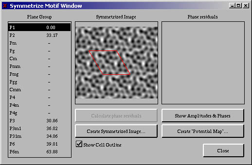
Which symmetry to use is a choice that you have to make – there are no rules which are always true. A reasonable suggestion is that if there are two (or more) symmetries with very similar phase residuals, the higher symmetry should be used. (It is more likely that instrumental effects reduce the apparent symmetry than increase it.)
One of the more significant sub-windows is launched by clicking on Create Potential Map (shown below using p6 symmetry). This will perform an approximate correction for the effects of the objective lens transfer using symmetry (see below). The phases from this corrected image can be used later in a Direct Methods analysis. (To copy phases, highlight the column and then either use CTRL-C or select Copy from the Edit menu. The program handles which phases go with which reflections automatically.) You can also change how the amplitudes are sorted by clicking on the top of the columns to sort by spacing (default) or amplitude. In order to activate the CTF correction, the image must be calibrated. The data is calibrated by giving the d-spacing for one of the reflections in the data set at the bottom of the window. Once calibrated, the resolution for the potential map can also be set which will influence the number of reflections which would be set in the "Adjusted" phase columns.
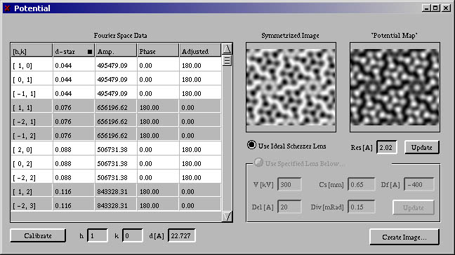
Note that if you previously calibrated the image, the lens characteristics will be available and accurate. You can now generate a larger tiled version of your symmetrized cell using the Create Image button. This image can be saved using the options in the File menu.
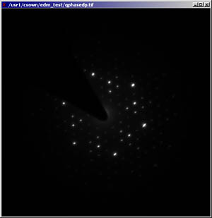
A second set of algorithms can be used to quantify intensities in a diffraction pattern using the central region of the main EDM menu.
The first step is to use G1, G2 and G3 to define 3 lattice points in quick succession using the targeting reticle and left-click. Then enter numbers into the fields next to G1, G2 or G3 (as appropriate) to specify the indices for each reflection. Pressing the Find button will then mark the lattice for you as illustrated in the two pictures below.
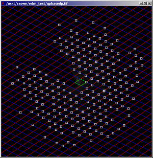
Moving below to the Peaks/Intensities section of the interface, you should first select a spacegroup to use. Note: all the possible two-dimensional spacegroups are included; if you are assuming kinematical scattering (or something close to it) you may want to limit yourself to the possible 2D Patterson symmetries (all of which contain an inversion center). After selecting this, you can press Find Peaks to find the diffraction intensity peaks in the lattice. You may want to adjust the correlation threshold for including more or fewer peaks. This value is in essence a cutoff for when the program will ignore a point. A suggested range of values will be output in the information field after you have done an analysis; you can delete the peaks then recalculate. Be careful not to set the value too low, or noise may be treated as a point and measured. The below right image shows the peaks found using the default threshold of 0.5.
There are two other important options for the Find Peaks function that specify how the intensities are found and measured. The "Int Meas" field contains a list of several different methods for evaluating the intensity of a peak. The "Criteria" field contains options for how classification of a peak (such as valid point vs. noise) is performed. You can use the Test button to see the R-factors for various space groups for evaluating how well the the symmetrized dataset fits the measured experimental data. Currently there is a hard cutoff point (R=0.15) under which a symmetry is highlighted as a "good" fit. The tables below contain details about the options for the peak-finding algorithm. The defaults are typically most accurate, but there are cases - such as if you have poorly-defined peaks of varying shapes - where the non-default options might work better. (Note: After peaks are located, the peak-finding controls will become greyed out until you press Delete Found Diffraction Peaks or select another image in a different window to measure.)
Note: the "E" button (Expert Mode) will allow you to change some of the controls for the measurements -- to be used cautiously.
Int Measurement
| XCF | This uses a cross-correlation function to fit an averaged peak against individual peaks. This is the most accurate method, with a couple of caveats:
|
| Integ | This integrates the total intensity within a square region around each spot. It is not as accurate as XCF. |
| IntegBZM | This integrates after removing a background and any pixels which are less than zero, a circular region around the spot. |
| IntegBZ | This integrates after removng a background and any pixels which are less than zero, a square region around each spot |
Criteria
| Image Mean | This uses the mean of the image as a criteria for selecting whether a spot is noise or might be a peak. If XCF is used, there is a second check (more accurate) for each spot. |
| Local Mean | This does the same as Image Mean, using a local mean around each spot. It is the default, probably the best. |
| Local Standard | Similar to above, using a standard-deviation test. |
| None | Uses all spots within the active region, which is most of the picture. |
Find Peaks will collect and store all peaks in the image measurable based on the above settings. After finding the peaks, you can now use the Quantify/Symmetrize button to convert the measurements into a list of numbers that will later be used by direct methods. This routine will generate a table (shown below) with the results (symmetrized if specified). The Friedel option, when checked, forces the algorithm to conduct symmetry averaging of Friedel pairs. If one member of the pair is not measured (for example, due to a beam stop), the single measured value is used for both reflections. For non-centrosymmetric structures (P1 and some P3 structures), make sure this box is deselected; when the Friedel option is not used, the software will generate the full set of reflections (i.e., includes both elements of a centrosymmetric pair present if both have been measured).
The Friedel and Group options should be specified right before quantifying/symmetrizing.
You can also display a symmetrized diffraction pattern, as well as the averaged spot motif that the program used. The latter is somewhat critical for accurate intensity measurements and later releases will include options for processing this motif prior to its use for quantification.
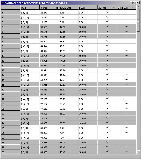
The columns in the table should be reasonably self-explanatory. Brief explanations are included in the following table:
| [h,k] | Denotes the index of the reflection. |
| d-star | The reciprocal length of the reflection (if uncalibrated, these values will have correct ratios to each other, but will have incorrect absolute values). |
| Amplitude | Contains the structure factor amplitudes measured by the program, and "Phase" contains the assigned phase of each respective reflection. |
| Phase | Known phase of a reflection. This column will be empty until you copy and paste real phases from high-resolution images (see the latter part of section 2) or you specify phases by hand. Insert phase information in a field by double-clicking and then typing in the value of phase when the type cursor appears. |
| Include | Allows you to select which reflections to include in the later Direct Methods analyses. |
| Use Phase | Specifies whether or not the phase will be fixed in Direct Methods (a phase is not included - i.e., guessed by Direct Methods - if this field is not checked). |
A simple phase extension can be run by copying phases that were generated from an averaged image (or by some other method) into the table of entries from quantification of a diffraction pattern – this was already done for the table shown earlier. (You can also jump directly here by reading an .hkl file from the main File menu.) In this case the program will try and read an .ins file, if it exists to find parameters such as the cell size (see later for information about file formats). After this, the Direct Methods window will open up a "Feasible Sets" submenu. Pressing Run Phase Extension will take the phases that you have provided and combine these with the intensities to try and find an improved map of the structure. (The program will complain if there are no phases, and will also complain if they are all set but you don't allow the phases to vary; in both cases there is no point in doing a phase extension!)
Some words of caution. Just because certain phases were found in the image does not mean that they are correct. Inaccurate values from beam or crystal tilt as well as astigmatism can have a large effect. You should try and be conservative, limiting yourself to reflections which correspond to relatively large spacing, are strong, and where you have confidence that the phase you found is close to correct.
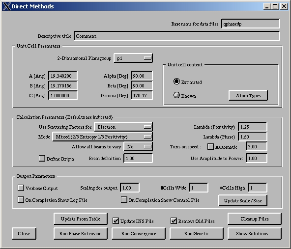
There are several parameters that can be adjusted; more information can be found in the documentation for fs98; the default parameters will work in most cases. One is the contents of the unit cell, which is used to estimate in absolute terms how strong the reflections are. The "unknown" option often works reasonably well with electron diffraction data, and normalizes based upon the sum of the intensities. Alternatively you can enter some values yourself. Experience indicates that in general it is better to overestimate the number of atoms than underestimate. In addition, if the sample is relatively thick (>30nm) you should use small temperature factors since higher angle reflections may have a noticeable dynamical component.
The symmetry that you choose in the 2D plane group field can also be critical. Glide planes and screw axes can lead to an apparent reduced symmetry, and inferior results. Unless you have the symmetry previously determined (e.g. from CBED) you should treat this as a variable and try different options.
One important point. With a very thin sample (e.g. 1nm) and very good phases (e.g. accurate to 10 degrees) you will get a very high quality map of the structure. In other cases not all atoms may show, and the peak heights may not be correct. Part of this can be due to channeling effects (dynamical diffraction), others are just intrinsic to Direct Methods. If the particular structure does not have relatively well-separated atomic columns along the beam direction, in general Direct Methods (in two dimensions) will not produce anything useful although phase extension might.
An alternative and more powerful method is to vary some of the other beams (for which the phases are not a-priori known) which is discussed in the next section.
Within the Feasible Sets menu, there are (at the bottom) commands for running a complete Direct Methods analysis. This is when you have either no phase information (or don't trust the phases you do have), or when only a few phases are already known. The procedure is slightly complicated, and is broken up into three sections. Note: by default the Remove Old Files checkbox is set, which will remove older data from previous runs. If you uncheck this you can continue an analysis that was done before but this can lead to unpredictable results if you are not careful and have not worked through the fine details of how fs98 works.
This takes the amplitude data and estimates which reflections are most significant in terms of their phases defining phases of other reflections. Note: any phases which are already included in the table are passed through so will be retained. For a complicated material, you can therefore use a few phases from HREM to help constrain the later results (and thereby get better results). It is possible to edit (by hand at the moment) the files which are created and determine how the genetic analysis is run; additional editing capabilities will be included in an "expert mode" at a later date.
The second step permutes using a genetic algorithm the values of some of the phases (the ones the convergence analysis decided were most significant) and finds the most feasible values. Please note the use of the word "feasible". What you are really doing is finding phases which are consistent with the presence of atoms with well-defined scattering potentials which give intensities similar to what was measured. Very often there is more than one possible solution; for instance, there is almost always the "Uranium Solution" where all the phases are 360 with just one atom. You have to use other constraints (e.g. chemical information, common sense) in the later analysis.
At the current moment this runs in your terminal (where you started EDM from) and can take some time, 10 minutes to several hours for a large dataset. You can monitor its progress by bringing your terminal to the foreground. In later releases options to run this as a background process will be included.
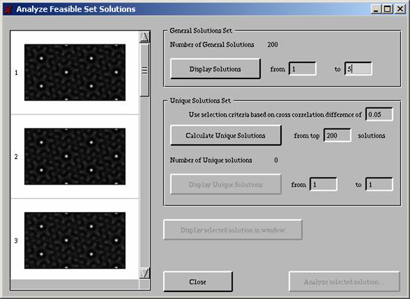
The Show Solutions button will open another window which will allow you to analyze the results. This is split into two parts. The first will calculate and display on the left the most feasible solutions, the number displayed being specified by the fields to the right. An example is given below. You can see a larger image of any of them by selecting, then clicking the Display button. (Note: the number of unit cells and magnification is controlled by values in the Direct Methods window; you have to use the update scale and size button so the Solution window knows that you have made changes.) In many cases several of the solutions will look similar, which means that they only vary in the phases of a few less important beams; this is a feature of genetic algorithms, part of the reason why they work well for global optimization problems.
More useful in general is to use the unique solutions. The program will calculate the top solutions (maximum 31) which are significantly different from each other based upon a cross-correlation test. A small value for this (e.g. 0.01) will permit very similar ones, a larger value (e.g. 0.1) only ones which are very different.
Going from a map to a structure is not a simple operation, and can easily go very wrong. To try and guide you through this you can select with the mouse any of the solutions and then click on the "Analyze selected solution" button. This will take you to the peaks menu.
This section is under construction
The sections below are intended to describe a fairly simple exercise which should teach you most of the features of using EDM. The various files referred to should come with your distribution of the software in the directory edm_test.
Explore this as appropriate.
The code should compile on any reasonably modern UNIX-based computer. A beta version for the Windows environment is available that should install itself, and seems to work on pentium based computers. If you run into problems, it is probably simplest to subscribe to the EDM listserver by sending an email to listserv@listserv.it.northwestern.edu_ with "SUBSCRIBE EDM Firstname Lastname" in the body of the text, then send an email message to users who may have encountered (and solved) similar problems.
Installation is fairly standard, following the general model for most GNU code. If you are not familiar with this (and/or do not have rights to install the software in the standard locations of /usr/local) you should get some assistance. It does require two other libraries, fftw and libforms. Many systems (e.g. linux) may already have libforms installed, and you may also have the fftw Fourier Transform libraries present.
To install the software from source code, you need to perform several steps of compilation:
Download the EDM source code if you do not already have it.
Unpack the code which is in a tgz (tar and gzip) form.
If you have root privileges, run the command "./configure" from within the directory you just created. If you don't have root privileges, in particular if you cannot create files in /usr/local, you can perform a local installation by typing "./configure --prefix=XYZ", where XYZ is the directory where you will install the code. Full details about the options can be obtained by typing ".configure --help" (see also below).
If a viable version of fftw or forms is not found on your computer, you will be asked if you want to compile them as well. (Note: the program looks for a single-precision version of fftw in either libsfftw or libfftw; you might only have the double-precision version on your computer.) If you have root access you may want to go directly to the fftw (and forms) directories, then use ./configure to install these yourself, but you don't have to. Note: within these subdirectories the default location where the code will be installed is /usr/local -- change this if appropriate. Also, be aware that the code looks for versions that are compatible with the compiler that you used, so if they were compiled with your native C you have to use this.
The script should run without problems, UNLESS your system is not well configured (e.g., you do not have a viable C++ compiler). By default it will look for and use the gnu compilers (since these are pretty much the same on all computers). It has been tested, reasonably well, with compilers on HPUX, SGI and SUN systems. Unfortunately the GNU compilers are much more tolerant than the C++ compilers on other systems, so minor "bugs", more accurately inconsistencies, are sometimes found with these other compilers. Since nowadays the gcc compilers are almost as fast as native compilers, it is probably simplest to use these.
The make command should run without problems. If it does not, please make sure it is not a configuration problem. For instance, if the configure script stops, saying that it cannot find a viable fortran (or c++, c) compiler, there is nothing we can do! Some useful commands are:
| make clean -k | This will clean up (large) .o files, continuing even on error. |
| make distclean -k | Also removes the Makefiles generated by ./configure (you need to do this if there was something badly wrong with a prior attempt. |
| ./configure -C | Use a cache file to speed up the configure. If something went wrong you need to use make distclean or delete config.cache since otherwise the (bad) parameters will be remembered. |
The code knows reasonably good flags for many system compilers, and will set these. You can always change these yourself by setting the standard compilation parameters:
| CC | C compiler command |
| CFLAGS | C compiler flags |
| LDFLAGS | linker flags, e.g. -L if you have libraries in a nonstandard directory |
| CPPFLAGS | C/C++ preprocessor flags, e.g. -I |
| F77 | Fortran 77 compiler command |
| FFLAGS | Fortran 77 compiler flags |
| CXX | C++ compiler command |
| CXXFLAGS | C++ compiler flags |
| CXXCPP | C++ preprocessor |
| CPP | C preprocessor |
If your X libraries are in strange places (that the script cannot find), try:
| --x-libraries=DIR | X library files are in DIR |
As a caveat, the LC_ALL variable can be critical if your computer is setup to display in a language other than English. In this case you need to set this to (depending upon your system) something like LC_ALL=C prior to running or compiling the code.
In addition to the standard compiler options, you may also want to use:
| --enable-ncemss | This will also install the NCEMSS multislice package |
| --enable-mbfit | This will also install the MBFIT CBED package |
| --enable-semper | This will also install some semper compatibility routines |
| --enable-focus | This will set "click-to-focus" mode as the default windows behavior. (This mode works best on all computers that we have tested EXCEPT for some Win32 machines where it can lead to bizarre behavior.) |
| --enable-shared | Flag for shared libs (dangerous!), default off |
| --enable-both | Flag to compile both forms and fftw, default off |
| --enable-forms | Flag to compile forms, default off |
| --enable-fftw | Flag to compile forms, default off |
| --with-gcc | Flag to use gcc, g++ and g77, default |
| --enable-debug | Flag to turn on debugging, default off |
You can use "--disable-XYZ" for these as appropriate to turn them off. A full listing can be found by using ./configure --help.
Perhaps the simplest way to use the code in a windows environment is to use cygwin, assuming that you have a reasonable amount of display memory. Download the distribution from www.cygwin.com, and install for certain the gcc and g77 compilers. Note: DO NOT INSTALL fftw since this is a more recent version. Then first, go into the fftw directory and install this (./configure ; make ; make install) then do the same for the forms directory (./configure ; make ; make install). It is recommended that in the top directory you then do "./configure --prefix=c:/cygwin/usr/local/edm" since this sets the path for the documentation correctly. After this "make ; make install" should work seamlessly.
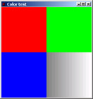 When you try to run EDM for the first time, if it does not run or is buggy, you might need to check your environment variables. A list of the required variables is given in the FAQ. Prior to using EDM, it is also a good idea to run "edm.exe -t" to bring up the test image (shown right) to test whether colors will be displayed properly on your system.
The Win32 version comes in two flavors, one with an X-server and one without. The former package is stand-alone and will run upon installation without any additional software. If you already have one of the commercially available X-servers (for example, StarNet X-Win32 or Cygwin), you should download the EDM version without the X-server and start your X-server before using EDM. EDM will not run unless your X-server is configured properly. EDM Win32 is built upon the Cygwin platform and the included X-server is derived from Cygwin's XWIN.EXE.
The Win32 installer installs the software by default into the C:\Program Files directory. Within the C:\Program Files\bin subdirectory, in addition to the EDM binaries there are several Unix utility executables that will run on a Win32 platform. SH.EXE is available for start a Unix-style shell, and from within this shell, you can do things such as use PICO.EXE to edit text files.
Upon first start of the X-server, the batch file will create a folder called ./tmp. This contains temporary information for the window server. The ./locale folder contains some fonts for the X-server; the server will not start up properly and will crash unless the fonts accessible (also applicable if you have Cygwin already and are using the X-server-less EDM with the X-Server from Cygwin).
When EDM is started, the front-end is launched from a DOS terminal window. Messages from Direct Methods analyses will appear here, as well as any error messages generated by the software. In addition, if you use one of the command-line switches to launch EDM, verbose information will also appear in this window. It is useful to be able to see messages in this window while EDM is running (likewise for the Unix versions).
Provides facilities for saving images, reading images, and saving or reading .hkl files. At the current moment, images can be read or saved as (uncompressed) tiff files or read as raw input in a number of different formats. If the program does not recognize an image as a tif file, it opens a window where information about the format can be included.
If you have a cygwin version, some additional commands will be present which will allow you to access some standard windows utilities, for instance wordpad and windows explorer
Standard cut, paste etc commands.
Provides a number of tools for performing simple image manipulations.
Opens up two menus for using fs98 Direct Methods. More information about the commands can be found in /usr/local/edm/html/fs98.htm.
Shows what windows have currently been opened.
Known Issues:
Possible Issues:
For the Win32 version, if I can't get the X-server or EDM to run via the windows shortcuts, what can I do?
If you know how to use DOS from the command line and edit batch files, you can try executing the software line-by-line from a DOS window. In Win32 operating systems, you can run "command.exe" from the start bar, or simply "cmd" in NT-based operating systems to bring up a DOS window. The first things to check are your environment variables (>echo $VARIABLENAME, see next question below). You should also check if the Cygwin mount points are properly established and pointing to the right places (>./bin/mount -m). EDM tends to work pretty robustly with Windows; most problems stem from issues with getting the X-server up and running and performing stably.
What environment variables need to be set in order to run the software?
The EDM and NCEMSS code use several environmental variables in order to determine where help information and executables are. These are set at compile time, so if the programs remain in the same location they can be ignored. Otherwise, if you relocate them they have to be adjusted and set (for instance in your startup script). They are:
| PREFIX | The location of the top directory where the code is. If unset, it defaults to what was used as the prefix during compilation (default /usr/local/edm). For cygwin you may need to use "export PREFIX=c:/cygwin/usr/local/edm" for the help to work correctly. |
| EDM_DOCDIR | This is added to the end of PREFIX to indicate where the html help files are located. If not set, defaults to "/documentation/". |
| EDM_BINDIR | This is added to the end of PREFIX to indicate where the executable files are located. If not set, defaults to "/bin/". |
| BROWSER | This is the full path to the web browser that will be used both to view images and help files. |
| NCEMSSDIR | The directory where global data for NCEMSS is kept |
| NCEMSSPOOL | The directory for files that should be available for all users, e.g. selected multislice atomic configuration files |
Note: it may be advisable to also set the PATH variable to ensure that EDM and NCEMSS are found.
For the windows environment, these are set in .bat files in the EDM directory, and the locale variable is also set to C. (You might need to set the locale in unix systems if you are not using English, since this determines the length of characters which both EDM and NCEMSS expect to be 8 bits.)
Why is the "right" solution not always the top solution that the Direct Methods code finds?
Direct Methods involve some statistical relationships as well as exploit as a-priori information that the diffraction pattern was created from a set of well-separated atom-like features. Dynamical diffraction can (it does not always) perturb this so the "right" solution is not always the top one; the code does not know (for instance) how much dynamical diffraction you had.
Some of the peaks where I expect to find heavy atoms appear weak in the maps?
Due to channeling (dynamical diffraction), at most reasonable thicknesses, say 10-20nm, heavy atoms (strictly speaking columns with a larger projected potential) may not scatter so much. This is similar to classic thickness fringes; the scattering from these columns have gone up to a maximum and come back down. In many cases lighter atoms, e.g. oxygen, can show up more clearly.
Do I need to have measured all the reflections – some are obscured by a beam stop?
No. The code is designed to handle cases where some of the reflections have not been measured, even very strong ones. If you think some of the reflections were incorrectly measured exclude them from your dataset.
How many beams should be varied in the Genetic Algorithms (GA)?
This is not a simple question. If too small a number is used, the GA will not utilize its capabilities to refine, so you will obtain a list of solutions without any clear winner(s). If too large a number is used, it may be that one solution will dominate at the expense of others. The code uses what it believes are reasonable numbers. If the top 50 solutions are all the same (and unphysical), you have probably used too many. To some extent the possibility to look at the unique solutions overcomes this. If in doubt, edit (by hand) the file control or adjust the variable CAMP which in part controls this in the divergence calculation.
I'm getting Patterson solutions -- why?
This can happen if the amplitude of reflections at higher angles is too large, for instance due to dynamical diffraction or (for surfaces) due to measurement errors of subsurface distortions. In this case you may want to reduce the angular resolution used; it is rarely that useful to go beyond a 1.0 Angstrom resolution initially unless the data is very accurate.
The map I'm getting appears to be the reverse of what the real structure is
This is called getting the Babinet solution, and can occur if you did not ask for enough atoms, and/or if there are substantial dynamical effects. (A solution of -F(hkl) for the structure factors is called the Babinet of F(hkl).) The "Babinet" command in the peaks control window is designed to allow you to explore whether this is what you have for an unknown structure.
Can EDM read semper files?
Not at the moment without a little difficulty due to the extra characters that fortran code puts at the end of a line. Code to read semper files will be added in the future.
Can EDM refine a structure for me?
Yes, but be careful! When dynamical diffraction effects are included it can become very difficult to find additional atomic sites that were not in the original map in an automated fashion. While the direct methods part of the code does not seem to care too much about dynamical effects, the refinement can be corrupted by them. Research is ongoing.
Can EDM output a .cif or files that can be read by other code such as SIR or Shelx?
Not yet, soon. The format is not that different.
Can EDM read files from Digital Micrograph or other companies which sell cameras?
If the files are standard tif, or some straightforward binary structure, yes.
What warranty is there that the results from EDM are right?
None. This is GNU software, distributed in the hope that it will be useful, but WITHOUT ANY WARRANTY; without even the implied warranty of MERCHANTABILITY or FITNESS FOR A PARTICULAR PURPOSE.
This section is under construction, sorry
This software started life as an attempt to produce a user-friendly version of some direct methods code. As the project developed, we decided that it would be useful to add a multislice code since with bulk electron diffraction one can never avoid dynamical effects, although in many cases they are not critical (to be specific, if 1s channelling dominates). We also decided to adopt a GNU model for the software to try and make it as standard, and widely usable as possible, avoiding have different versions for specific operating systems. The hope is that in a few years the code becomes something which is widely used and maintained by the electron microscopy community as a whole.
It will, of course, be some time before the code reaches this stage. We hope that others will be interested in contributing, for instance specific code, suggestions or time to test it in different environments.
If you are interested in contributing code, there are some basics that need to be adhered to. The code should be something which is generally useful and can be applied to either (or both) images and diffraction patterns via a GUI. The code should be standard C, C++ or Fortran and should (as a minimum) have been tested with the GNU compilers to make sure it does not have incompatible features. It should have a Makefile (configure scripts would be better), help information in terms of html files and NOT require an extensive set of specialized external libraries to run. (The more external libraries are required, the harder it becomes to port it to different computers and to maintain.) You have to be prepared to provide source code (a basic GNU point), and help to maintain it.
If you want to contribute, please contact either Laurie Marks or Roar Kilaas. No promises; we will do our best. Some possibilities are: